

Generalisation in Neural Networks
What is Generalisation?
In statistical learning theory, generalisation is a measure of the extent to which a statistical model can extrapolate. For example, a model fitted with a finite set of points that interpolates these points has a low capacity for making inferences regarding points that lie outside of this finite set. Such interpolatory behaviour is referred to as overfitting and arises when a model focuses too heavily on the intricate details of a data set. On the other hand, underfitting arises when a model is too broad in its representation and cannot capture the details of a data set. Techniques in classical statistics have been thoroughly investigated to understand when overfitting, or underfitting may occur and have consequently been refined to mitigate these phenomena in practice. It is widely understood that the parameter count of classical statistical models causes the emergence of these phenomena. In particular, having an over-parameterised model, that is a model with more parameters than data points, leads to a model that overfits.
However, neural networks do not conform to the classical paradigm of statistics, and thus their relationship with generalisation is more nuanced.
Fitting, or training, a neural network involves using training data to manipulate its parameters, usually through gradient descent, to arrive at a function that accurately represents the distribution from which the training data was drawn. A priori the distribution from which the training data is drawn is unknown, however, it is assumed that the empirical distribution of the training data is close to the underlying distribution. Indeed the training data is assumed to be an independent and identically drawn sample.
The training process of a neural network is driven by quantifying the network performance on the training data using a loss function. Usually, one does not train a neural network with all of the available data but holds out a set to test the neural network. Therefore, in the context of neural networks we can quantify generalisation as the difference between the loss function of the network on the training set and the loss function of the network on the test set.

Experimental Evidence
With the rise of neural networks, we are at a stage where neural networks tend to be heavily over-parameterised. To the extent that neural networks can achieve low training errors even on data with randomised labels. Hence, the problem of underfitting is not prevalent for neural networks, whereas overfitting is still a cause for concern. However, in practice, even though neural networks are over-parameterised they have a remarkable ability to learn general representations of the training data. This does not conform to classical statistical learning theories, and so requires more sophisticated modes of analysis.
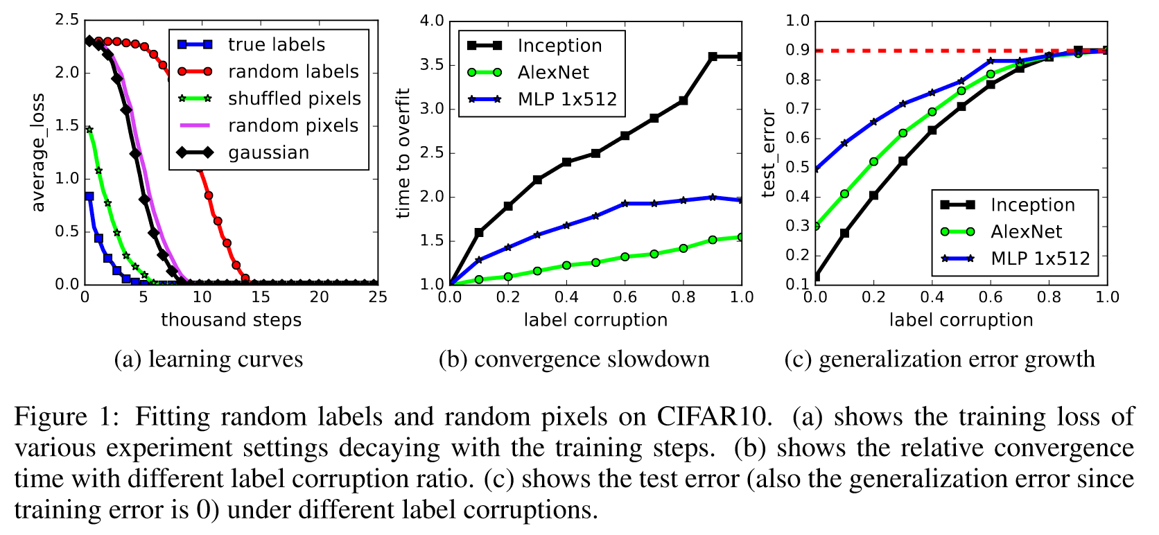
Consider the Figure 1 from [2]. It shows how an over-parameterised neural network can overfit, but when presented with structured data it develops a general representation.
What we see in Figure 1(a) is that the training loss of a neural network eventually decreases to zero, even when the data points are randomly labelled. As expected training loss decreases fastest when the data has its true labels as the network can exploit the structure of the data to inform meaningful representations. As the training loss on random labels also decreases to zero we deduce that the neural network can overfit to the data.
Figure 1(b) makes the conclusions from Figure 1(a) more explicit by showing that the time it takes the neural network to overfit monotonically increases with the amount of randomness present in the data set.
Figure 1(c) shows that the representation learned by the network becomes less general as the amount of randomness in the training data increases. This is to be expected, as with random data no structure can be exploited to make inferences on unseen data.
Formalising Generalisation
Neural network generalisation can be investigated empirically or theoretically. The empirical approach involves deriving statistics that correlate with generalisation error. The theoretical approach, or at least the one we consider here, involves deriving probabilistic bounds on the generalisation error. Despite the approach one takes to explaining generalisation, both target at least one of the components of neural network generalisation, namely the training data, the learning algorithm, or the neural network architecture.
The Probably Approximately Correct (PAC) learning framework provides probabilistic guarantees on the performance of trained networks. More specifically, given a model, which we will take be a neural network, a training algorithm and a set of training data, PAC bounds are of the form
and hold for a specified probability.
The true error refers to the discrepancy between the neural network representation and the underlying distribution of the data. As the underlying distribution is unknown we want to bound this quantity by other quantities that we can compute.
The train error refers to the discrepancy between the neural network representation and the training data. We can directly compute this quantity, and it is the metric that governs the training process of a neural network.
The complexity term is dependent on the neural network architecture, the learning algorithm, the training data and the confidence with which one wants the bound to hold. It can be thought of as an inverse measure of the generalisation capacity of the trained neural network. That is, a low complexity term reflects that the training error is a good proxy for the true error, meaning that when a neural network achieves a low training error we can be confident that its representation of the data extrapolates beyond the training data. A lot of the research regarding neural network generalisation is in optimising this complexity term, as in most cases a neural network can achieve a very low, often zero, training error. For classical statistical models, the complexity term involves quantities such as the Vapnik–Chervonenkis (VC) dimension, the number of parameters in the model, or the Rademacher complexity of the training data. However, for modern neural networks that are heavily over-parameterised, this quickly leads to vacuous bounds that are not useful in practice. Indeed VC dimension is bounded below the number of parameters in the model [3], and so even for relatively small networks the bounds are not useful.
PAC-Bayes refer to a PAC bound that is derived under the Bayesian machine learning framework. Typically, a prior distribution is set over the parameters of the neural network, and then a posterior is formed using the learning algorithm and data set. The complexity term in this case is then also dependent on the properties of the posterior and its relationship to the prior distribution.
Optimising PAC-Bayes Bounds
Due to the unsuitability of conventional metrics for generalisation, an alternative approach is required to derive non-vacuous bounds for neural networks. From empirical studies, it is thought that stochastic gradient descent, the learning algorithm used for training neural networks, has an implicit regularising effect on the learned representation of neural networks [1]. Thus to develop non-vacuous bounds for over-parameterised neural networks [3] takes the Bayesian perspective of the PAC learning framework to harness the stochasticity of stochastic gradient descent and facilitate the optimisation of the complexity term through the posterior distribution. More specifically, [3] operates under the intuition that stochastic gradient descent finds good representations if they are surrounded by a large volume of similarly good solutions. Therefore, given a prior over the neural network parameters, the optimisation algorithm proposed by [3] determines a posterior distribution over the neural network parameters that minimises the complexity term, with the intention that the resulting generalisation bound is not vacuous.
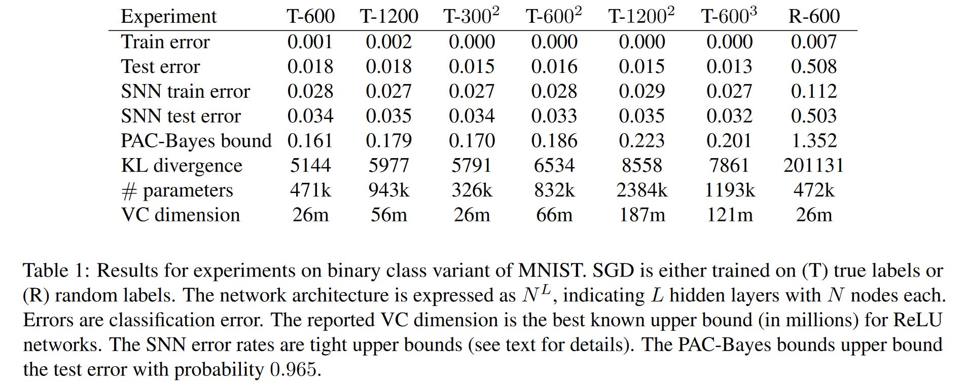
From Table 1 of [3], we see that the PAC-Bayes bound are non-vacuous for the majority of cases, however, it becomes vacuous when the neural network is trained on random labels. Although we do not expect, or even do not want, the neural network to learn a general representation of the set of random data we would like the generalisation bound to be vacuous. As the task presented to the neural networks of Table 1 of [3] are binary classification tasks, we would expect any reasonable model to perform better than random guessing and achieve a test error of around 0.5. Indeed this is exactly the case for the test error of R-600. Furthermore, observing the behaviour of the PAC-Bayes bound it seems to be largely governed by the size of the neural, which although a key component to generalisability other facts of the neural network should influence the bound.
The authors of [3] realise the sub-optimality of their bound, but one should appreciate that their work provides initial evidence that vacuous generalisation bounds for neural networks are achievable in practice. Future directions of refinement include a better understanding of the role of stochastic gradient descent on generalisation and identifying the more prominent features of the neural network architecture that contribute to an ability to generalise.
Compressing Neural Networks
One can intuit that generalisation is an essentially equivalent concept to compression. That is, being able to effectively compress data is akin to identifying high-level features that facilitate the reconstruction of the data. Consider, the laws of physical motion. By realising that the force an object experiences is related to the acceleration it experiences, one can determine the trajectory of a projectile. Thus, one has compressed the dynamics of all moving objects into a single equation. However, this compression is perhaps too strict. Indeed, this relationship between mass and acceleration ceases to hold at the scale of the cosmos. Thus there is a balance between the level of compression and the subsequent generalisability.
With this physical example, it is clear that understanding compression mechanisms helps elucidate the underlying mechanisms governing a set of data or processes. With this realisation [4] attempts to gain more insight into neural network generalisation, something the bounds of [3] fail to provide, by understanding how neural networks can be compressed whilst experiencing minimal losses to performance.
To derive its compression algorithms, [4] investigates the stability of neural networks when noise is injected into the inputs at different layers through the network. It is reasonable to assume that if a neural network is stable to noise then it has learned a robust representation for the data. For example, even if our measurement of an object's acceleration is slightly inaccurate our model is still able to determine a reasonable value for the force the object experiences experiences. Note that stability is not necessarily dependent on the actual data, instead it pertains to how the neural network operates on the data.

On the left of Figure 4 from [4], we can see how much tighter the generalisation bound obtained through this compression approach is compared to other generalisation bounds, for this particular scenario. Moreover, from the right of Figure 4 from [4], we see how the behaviour of the bound more closely matches the generalisation error of the neural network during training. However, we note that towards the latter epochs, the correlation between the generalisation bound and generalisation error decreases. The authors of [4] link the deterioration to the point when the neural network achieves zero training error. Therefore, their bound does not fully explain the generalisation of neural networks and so there is still work to be done to try and fully explain neural network generalisation.
Other Approaches
Recall, that explaining neural network generalisation requires understanding the training data, the learning algorithm, and the network architecture. The work of [3] focuses on the implicit regularisation capacity of stochastic gradient descent to optimise the complexity term of a PAC-Bayes bound. On the other hand, [4] investigates the stability of the trained structure of a neural network to understand how general its representation of the data is. Both [4] and [3] do not emphasize the training data component of neural network generalisation.
The neural tangent kernel [5] is an interesting approach to explaining neural network generalisation that focuses more strongly on the training data compared to other approaches we have considered. The neural tangent kernel describes the local dynamics of a neural network during training and helps study the effects of depth and non-linearity on the generalisation capacity of neural networks [5].
Generalisation in Graph Neural Networks
Generalisation for Graph Data
Graph neural networks are architectures which capitalise on the inherently non-Euclidean nature of graph data. In large part, this involves facilitating the communication between nodes through their edges. Such mechanisms allow for information to be propagated through the network and are indeed referred to as the message-passing process. With these frameworks comes a capacity to deal with data that possesses non-standard topologies. For example, graph neural networks have become ubiquitous for performing inference on molecular data, where atoms are represented by the nodes of the graph, and the chemical bonds are represented by the edges of the graph.
However, this non-Euclidean and discrete aspect of the data means that the underlying assumption and techniques of PAC-learning do not easily transfer to this domain. Moreover, the intricate architectures of graph neural networks mean that structural arguments, such as compression and spectral theory, to explain neural network generalisation are more delicate in the case of graph neural networks.
Moreover, on the graph domain, there exist different levels of tasks. Some tasks exist at the node and edge level, such as the classification of nodes, the existence of edges, or the regression of node feature vectors. On the other hand, some tasks exist at the graph level, such as the classification of graphs or regression of graph-level statistics. Consequently, it is important, when speaking of generalisation, to be clear at which level we are operating as each level must be dealt with differently.
At the graph level things are relatively easy as one can consider each graph as a single data point, and with graph-level statistics, one can embed these points into some Euclidean space. From here all the tools from feed-forward neural networks become applicable. At the node and edge level, we encounter the issues of non-Euclidean and discrete domains mentioned previously.
Experimental Evidence
It is also essential to distinguish between the levels of tasks, as at each level the notion of overfitting is slightly different. At the graph-level generalisation is in the sense encountered for neural networks. However, at the node and edge level, one can speak about overfitting to the graph structure in addition to overfitting to the regression or classification tasks being trained for. More specifically, in some instances, the graph structure of the data provides no utility in performing the desired task. Consequently, due to the inherent architecture of graph neural networks and the fact that over-parameterised graph neural networks can overfit to graph structure, it is possible that the graph neural networks focus too strongly on the topology of the data and thus inhibit its performance on the desired task.

Consider Table 1 from [7]. It shows that for certain datasets, when a graph neural network is trained on the same data with its graph-structure omitted its performance increases from when the same graph neural network is trained on the same data but with the graph-structure included. This is evidence of the fact that the graph neural networks overfit the graph structure and thus experience a decrease in performance. These results are specific to the datasets but show that despite some data living in a graphical domain it does not mean that a graph neural network should be, naively, used to perform tasks on the data.
Augmenting Existing Ideas
Initial work by [6] and subsequent work by [8] extends the PAC-Bayesian framework from neural networks to graph neural networks. More specifically, they look at graph-level tasks such that they can treat each graph as a point sampled from an underlying distribution. As recognised by [8], a naïve application of generalisation bounds from neural networks to graph neural networks introduces a term that scales as
where n is the number of nodes in the graph and l is the number of layers in the graph neural network. Thus, such a naïve analysis is practically insufficient as the bounds quickly become vacuous. The structure of the graph neural network needs to be considered to refine the bound.
In [6] the maximum node degree of the graph is used to infer the generalisation ability of the graph neural network. Consequently, their generalisation bound scale with
where d is the maximum degree of the graph and l is the number of layers of the graph neural network. This can be seen as a work case analysis, and indeed the authors concede that the practical behaviour of graph neural networks is still unexplained by their generalisation bound.
However, the analysis made in [6] set the groundwork for others to conduct more refined analyses. In particular, [8] augments the work of [6] by an approach inspired by [4]. As a result, [8] develops bounds that scale with the spectral norm of
where P is the diffusion matrix of a graph and l is the number of layers of the graph neural networks. Consequently, [8] can derive a measure of the generalisation gap using the Hessian matrix of the loss function evaluated on the training data, with respect to the parameters of the graph neural network. Experimentally, it is shown that this measure aligns with graph neural networks in practice, and so the refined analysis of [8] indeed extends the limits of the analysis conducted by [6].

However, there is still work to be done to consider node-level tasks. Such tasks can be thought of as self-supervised tasks, where one has access to a portion of the node and edge features and is tasked with inferring information about the other nodes and edges. Extending the work of [8] to this setting is non-trivial as graphs are finite and so arguing in terms of expectations becomes more difficult. Instead [8] suggests that in this setting graphs should be viewed as a random sample from some larger graph, and then one can argue in terms of expectation on this larger graph.
Bibliography
[1] Neyshabur, Behnam, Ryota Tomioka, and Nathan Srebro. ‘In Search of the Real Inductive Bias: On the Role of Implicit Regularization in Deep Learning’. arXiv, 16 April 2015. [https://doi.org/10.48550/arXiv.1412.6614](https://doi.org/10.48550/arXiv.1412.6614).
[2] Zhang, Chiyuan, Samy Bengio, Moritz Hardt, Benjamin Recht, and Oriol Vinyals. ‘Understanding Deep Learning Requires Rethinking Generalization’. arXiv, 26 February 2017. [http://arxiv.org/abs/1611.03530](http://arxiv.org/abs/1611.03530).
[3] Dziugaite, Gintare Karolina, and Daniel M. Roy. ‘Computing Nonvacuous Generalization Bounds for Deep (Stochastic) Neural Networks with Many More Parameters than Training Data’. arXiv, 18 October 2017. [https://doi.org/10.48550/arXiv.1703.11008](https://doi.org/10.48550/arXiv.1703.11008).
[4] Arora, Sanjeev, Rong Ge, Behnam Neyshabur, and Yi Zhang. ‘Stronger Generalization Bounds for Deep Nets via a Compression Approach’. arXiv, 26 November 2018. [https://doi.org/10.48550/arXiv.1802.05296](https://doi.org/10.48550/arXiv.1802.05296).
[5] Jacot, Arthur, Franck Gabriel, and Clément Hongler. ‘Neural Tangent Kernel: Convergence and Generalization in Neural Networks’. arXiv, 10 February 2020. [https://doi.org/10.48550/arXiv.1806.07572](https://doi.org/10.48550/arXiv.1806.07572).
[6] Liao, Renjie, Raquel Urtasun, and Richard Zemel. ‘A PAC-Bayesian Approach to Generalization Bounds for Graph Neural Networks’. arXiv, 14 December 2020. [https://doi.org/10.48550/arXiv.2012.07690](https://doi.org/10.48550/arXiv.2012.07690).
[7] Bechler-Speicher, Maya, Ido Amos, Ran Gilad-Bachrach, and Amir Globerson. ‘Graph Neural Networks Use Graphs When They Shouldn’t’. arXiv, 8 September 2023. [http://arxiv.org/abs/2309.04332](http://arxiv.org/abs/2309.04332).
[8] Ju, Haotian, Dongyue Li, Aneesh Sharma, and Hongyang R. Zhang. ‘Generalization in Graph Neural Networks: Improved PAC-Bayesian Bounds on Graph Diffusion’. arXiv, 23 October 2023. [http://arxiv.org/abs/2302.04451](http://arxiv.org/abs/2302.04451).